If you have previously attempted to analyze NFL data, it is likely that you have tried to scrape ESPN or football-reference, which provides a wealth on statistics surrounding game data. However, if you ever wanted to obtain truly in-depth data, then it is likely that you found yourself leveraging the API maintained by NFL.com. Unfortunately, it’s data is surfaced in a JSON format that leaves a lot to be desired (i.e. it’s a nightmare). Lucky for me, I was recently scrolling through my Twitter feed and came across an interesting mention of a new R package called nflscrapR. After some exploration, I came through this quote from the author of the package:
NFL fans and sports enthusiastic alike, I would like to introduce the nflscrapR package, an American football data aggregator that will scrape, clean, and parse play-by-play data across games, seasons, and careers.
The nflscrapR essentiallys surfaces all play-by-play data for the last 7 seasons, and this has motivated me to start a deep dive on NFL data. I plan to have two main topics, one that focusses on players at specific positions, and another focussing on team dynamics and patterns. To kick this series off, we will begin with an exploration into the performance of NFL’s best running backs.
1. Prerequisites
In order to reproduce the figures below, wou will need to have R (v3.2.3 or above) installed on your machine. There are also a couple of additional libraries that will be required. Details on how to install those are shown in the commands below.
# install.packages('devtools')
library(devtools)

#> Skipping install for github remote, the SHA1 (05815ef8) has not changed since last install.
#>   Use `force = TRUE` to force installation

devtools::install_github(repo = "maksimhorowitz/nflscrapR", force=TRUE)
2 Collecting the Data
With the nflscrapR library now installed, you are now ready to collect play-by-play data for the 2016-2017 NFL season. Start by loading the library and collect the data using the command below:
# Load the package
library(nflscrapR)
library(ggplot2)
library(dplyr)
library(pheatmap)

# Collect data for 2016 NFL season
pbp_2016 <- season_play_by_play(2016)
Overall the pbp_2016 dataframe contains 100 data points for 45,737 plays, but for the purpose of this post, we will be focussing exclusively on fields related to running backs (In future posts, we will explore data relevant to other positions on the football field). In addition, we’ll focus primarily on frequently used running backs, which we empirically define as any player that has had at least 200 rushes over the course of the 2016-2017 season.
# Get all players with at least 200 rushes during the season
min_rush_cnt <- 200
rush_cnt <- pbp_2016 %>% filter(PlayType == 'Run') %>%
                         group_by(Rusher) %>%
                         summarise(rush_cnt = n(),
                                   total_yards = sum(Yards.Gained),
                                   mean_yards = round(mean(Yards.Gained), 2)) %>%
                         filter(rush_cnt >= min_rush_cnt) %>%
                         arrange(desc(rush_cnt))

# Get all rushing data for eligible players
rushing_stats <- pbp_2016 %>%
                 filter(PlayType == 'Run' & Rusher %in% rush_cnt$Rusher & Yards.Gained <=50) %>%
                 filter(down!=4 & !is.na(down)) %>%
                 filter(!is.na(RunLocation))
Altogether, we find that a total of 19 players rushed over 200 times during the 2016-2017 season. A short summary of their performance is show below.
3. Who are the most consistent and productive running backs?
When talking about the overall performance of running backs, it is common for people to report the total number of yards that were rushed for, or the average yards per run. While these are perfectly acceptable numbers to share, I’ve always felt like they did not tell the whole story. For example, a player could have a high average yards per run, only for us to realize that he actually often loses yards on a run but makes up for it with a few very long runs. Therefore, I started by looking at the overall distribution of number of yards gained/lost for each play, with the hope that this would reveal whether some players were more consistent on a play-by-play basis than others. We can use the ggplot2 library to generate a density plot of yards gained per play for each of our eligible players:
# Compare distribution of rushes for eligible players
ggplot(rushing_stats, aes(x = Yards.Gained, y = Rusher, fill=Rusher)) +
       geom_joy(scale = 3) +
       theme_joy() +
       scale_fill_manual(values=rep(c('gray', 'lightblue'), length(rushing_stats$Rusher)/2)) +
       scale_y_discrete(expand = c(0.01, 0)) +
       scale_x_continuous(expand = c(0, 0)) +
       theme(legend.position="none") +
       labs(x="Yards gained per play" ,y="")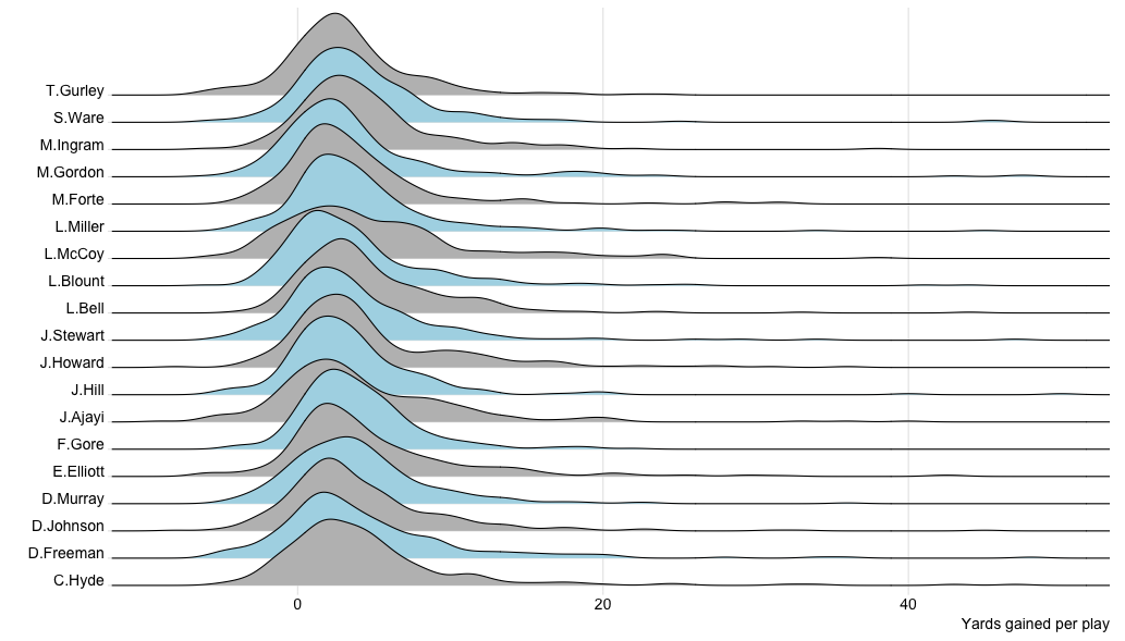
Overall, we see that most running backs have a similar distribution of yards gained by run. However, we can see that LeSean McCoy (7th distribution from the top) has a much “flatter” distribution (i.e. more variance in the distribution of yards gained per run), meaning his performance can be a lot more variable/unpredictable for any given run.
4. When are running backs used?
Another statement that is also commonly reported is that running backs are primarily used in early downs. To verify whether this is generall true, we can compute the total amount of runs that each player made across different downs, and go even further by breaking this down by quarter too. The code chunk below counts the number of runs that each rushing back made during pairs of downs and quarters.
# Compare when rushers are used
usage_stats <- pbp_2016 %>% filter(!is.na(down) & Rusher %in% rush_cnt$Rusher & qtr!=5) %>%
                             group_by(Rusher, down, qtr) %>%
                             summarise(cnt = n()) %>%
                             mutate(qtr_down = paste("Q", qtr, "- Down: ", down, sep=""))
We can then leverage the d3heatmap to quickly generate a simple heatmap of how often running backs are used during specific downs and quarters.
library(d3heatmap)

# pivot dataframe
usage <- usage_stats %>% dcast(Rusher ~ qtr_down, value.var = "cnt")

# clean data
row.names(usage) <- usage$Rusher
usage <- usage %>% select(-Rusher)
usage[is.na(usage)] <- 0

# normalize data
usage_norm <- t(apply(usage, 1, function(x) x/sum(x)))

# plot heatmap of proportions of rushes by different field locations and gaps
p <- d3heatmap(usage_norm,
               colors="Blues",
               Colv=FALSE,
               show_grid=3)

saveWidget(p, file="rusher_usage_down_quarter.html")
Proportion of rushes per quarter and downs for NFLs best running backs
In the plot above, we are essentially plotting the usage of each running back as a function of what stage of the game we are in. As we can see, it is abundantly clear that running backs are primarily used in the first two downs, and rarely during the third and fourth downs. Overall, there does not appear to be significant differences between how players are used. However, it does not answer whether some running backs perform better on certains downs, which is what we will address now.
5. Are some running backs better on certain downs?
Another question we can ask ourselves is whether some running backs perform better on later downs. To visualize this data, we can again generate a density plot of yards gained per play for each of our eligible players, while also facetting the data by downs.
# Compare distribution of rushes by downs
ggplot(rushing_stats, aes(x = Yards.Gained, y = down)) +
       geom_joy(scale=1, rel_min_height=.03, fill='black') +
       scale_y_discrete(expand = c(0.01, 0)) +
       xlab('Value') +
       facet_wrap(~Rusher, scales='free', ncol=3) +
       theme_joy() +
       theme(axis.title.y = element_blank())+
       labs(x="Yards gained per play" ,y="Down")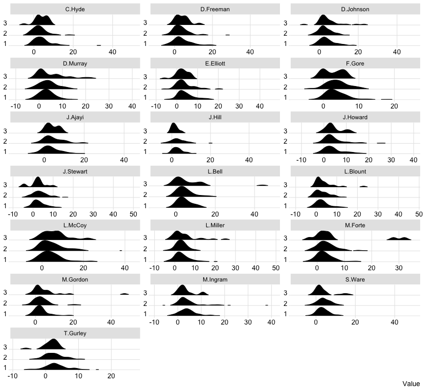
Again, we do not see any striking differences between players and the distribution of yards gained by down. However, it is interesting to note that most “long runs” (10 yards or above) tend to occur on the first down. When we look closely, we can also see that some rushers such as DeMarco Murray do exhibit visual differences between yards gained by downs. In this case, the “mass” of yards gained on the third down is much closer to zero than when compared to the “mass” for the first and second downs, which suggests that he may struggle during this down (this could be attributable to many factors: stamina, weaker offensive line on 3rd downs, etc…)
6. Where do the best running backs run?
It is fairly well accepted that the performance of a running back will be heavily influenced by the strength of the offensive line in front of them. With that in mind, let’s start by looking at the field location in which different running backs prefer to run. The plot below shows the number of yards gained by each running back based on which side of the field they ran towards (left, middle or right).
ggplot(data=rushing_stats, aes(x=RunLocation, y=Yards.Gained, color=RunLocation)) +
       geom_jitter(position=position_jitter(0.2)) +
       stat_summary(fun.data=mean_sdl, mult=1,
                    geom="pointrange", color="black") +
       scale_color_brewer(palette="Dark2") + theme_minimal() +
       facet_wrap(~Rusher)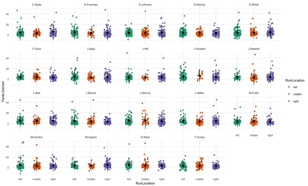
We can take this further by looking at the field location in which different running backs prefer to run. This can be achieved by generating a matrix that contains the proportion of rushes by field location for each player.
# Get proportions of rushes on different field locations
rush_locations <- rushing_stats %>% filter(PlayType=='Run') %>%
                                    filter(!is.na(RunLocation)) %>%
                                    group_by(Rusher, RunLocation) %>%
                                    summarise(rush_cnt = n()) %>%
                                    mutate(freq = rush_cnt / sum(rush_cnt))

loc_mat <- rush_locations %>% dcast(Rusher ~ RunLocation, value.var = "freq")
row.names(loc_mat) <- loc_mat$Rusher
loc_mat <- loc_mat %>% select(-Rusher)
The content of the loc_mat matrix contains the preferred rush locations of each running back, and can be plotted as a clustered heatmaps using the pheatmap library in R.
# Plot heatmap of proportions of rushes by different field locations
pheatmap(loc_mat, border="white", color = brewer.pal(9,"Blues"), cluster_cols=FALSE)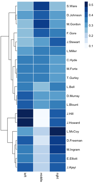
The plot above highlights which running back are most similar in their run locations. Rushers such as J. Ajayi, E. Elliot and M. Ingram, clearly avoid running in the middle of the field. On the flipside, rushers such as M. Gordon D. Johnson, S.ware and F. Gore clearly prefer running down the middle rather than to the sides. These patterns could be attributed to the running styles of each rushers (speed, mobility, strength etc…), but also the strength of the offensive line at particular positions.
7. Who creates the gaps for the running backs?
We can also explore the number of yards gained by each running back based on the offensive line positions that created space for them.
ggplot(data=rushing_stats %>% filter(!is.na(RunGap)), aes(x=RunGap, y=Yards.Gained, color=RunGap)) +
       geom_jitter(position=position_jitter(0.2)) +
       stat_summary(fun.data=mean_sdl, mult=1,
                    geom="pointrange", color="black") +
       scale_color_brewer(palette="Dark2") + theme_minimal() +
       facet_wrap(~Rusher)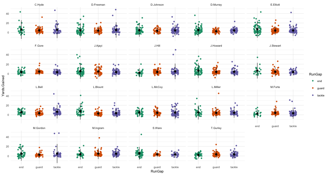
The proportions of run opportunities that was enabled by each offensive line position can also be summarized in a matrix using the command below.
# Get proportions of gaps created by different offensive line positions
rush_gaps <- rushing_stats %>% filter(!is.na(RunGap)) %>%
                               filter(!is.na(RunGap)) %>%
                               group_by(Rusher, RunGap) %>%
                               summarise(rush_cnt = n()) %>%
                               mutate(freq = rush_cnt / sum(rush_cnt))

gap_mat <- rush_gaps %>% dcast(Rusher ~ RunGap, value.var = "freq")
row.names(gap_mat) <- gap_mat$Rusher
gap_mat <- gap_mat %>% select(-Rusher)
# Plot heatmap of proportions of rushes by different field gaps
pheatmap(gap_mat, border="white", color = brewer.pal(9,"Blues"), cluster_cols=FALSE)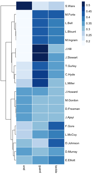
Again, we see many differences among the leagues top running backs. Unsurprisingly, a number of players have the most run opportunities created by the guard position, but a few players such as F. Gore, L. McCoy and D. Johnson run in gaps created by the tackle position. Finally, S. Ware from the Kansas City Chiefs often runs through gaps created by tight ends, which may be more representative of the team’s formation.
Conclusion
In this introductory post, we have explored the performance and patterns of some of NFL’s best running backs. Overall, it was a fairly superficial analysis, as it never considered interactions with other components of the team, or temporal patterns, but it does show the depth and power of this data. In the next series, I will dive into the performance and behavior of wide receivers, so stay tuned!