Rental Prices in the US
As a fortunate resident of New York City, I get to enjoy the many activities offered by a city that never really turns off its lights. The price to pay for such entertainment, however, are the crazy rental fees. I have stopped counting the number of conversations I have had with friends about some of the exhorbitant living costs in NYC. I have also drooled over multi-million mansions with sprawling views of the city, and wondered how studios the size of a shoe box could claim such high prices. Fortunately for me, I have been living in the same spot for the last few years, but am now expecting to start looking again soon.
This means that I am starting to look for both a new neighborhood and a new apartment, and for that I have been primarily relying on the Streeteasy and Zillow wesbites. Eventually, keeping track of all this gets a little confusing, and I can only imagine how much worse it gets for people just moving into NYC.
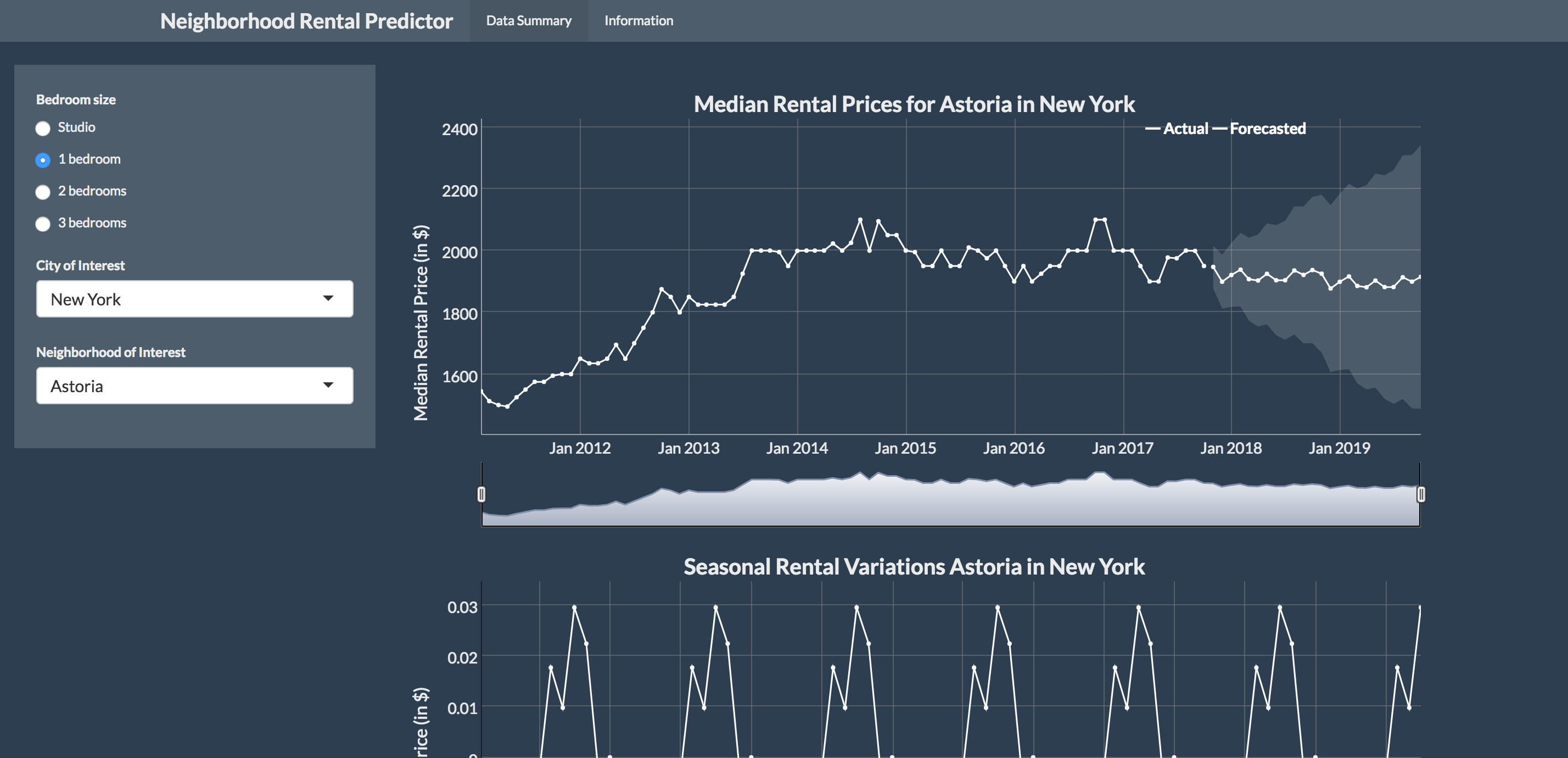
For these reasons, I decided to see if I could leverage some open-source data in order to extract and visualize some information out of it. In the following post, I will collect and analyze some of the great data made available by Zillow, while also going through the steps that allowed me to create the web application displayed below
Obtaining Zillow data & Forecasts
Obtaining the data for this project is very straightforward, and does not require any scraping or cleaning. All the data can be directly downloaded from the following link, and contains monthly median rental prices in neigborhoods of various US cities between 2010 and now. In order to produce forecasts of the time series represented in the Zillow dataset, I leveraged the additive HoltWinters function, which comes as part of R’s core packages). Briefly, the additive Holt Winters model assumes that the value of a time series \(Y\) at time \(t\) can be represented as:
where \(b_{1}\) represents the base signal of the time series, \(_{2}\) denotes the linear trend component, \(S_{t}\) is the additive seasonal factor and \(\epsilon_{t}\) is the random error component of the time series. The Holt Winters additive seasonal model assumes that the amplitude of the seasonal component of the time series is independent of the average level of the series itself. I thought that this assumption fit well with the Zillow data, so decided to work with that. I also assessed other methodologies for time series forecasting, but it eventually turned into a bigger project than I had intended. Instead, I have planned to write a comparative analysis for the various time series libraries available in both Python and R. In the meantime, let’s show how the app was built!
Building the Rental Predictor Shiny application
The next step was to build a Shiny app that allows anyone to look at forecasts and seasonality of different neighborhoods. For simplicity, I have hosted the app on shinyapps.io, but in order to ensure full reproducibility, I have containerized the full application using Docker. If you have not used or heard of Docker, their own website gives a very good description:
Docker containers wrap up a piece of software in a complete filesystem that contains everything it needs to run: code, runtime, system tools, system libraries – anything you can install on a server. This guarantees that it will always run the same, regardless of the environment it is running in.
With that in mind, the development workflow used to create this Shiny app was:
- Build the shiny app locally (i.e. on your local machine) and ensure that everything works just as expected.
- Create a file called
Dockerfile, in which we specify all the required instructions and commands, environnment variables and configurations. - Build and run the
Dockercontainer to check that the app behaves as expected. If not, iterate over the first step until you are satisfied. - Reap the benefits of a fully reproducible app that can be ran on any OS platform!
The source code for the full web app can be found at the following GitHub repository, and has the following directory structure:
.
├── Dockerfile
├── LICENSE
├── README.md
├── app
│   ├── data
│   │   ├── Neighborhood_MedianRentalPrice_1Bedroom.csv
│   │   ├── Neighborhood_MedianRentalPrice_2Bedroom.csv
│   │   ├── Neighborhood_MedianRentalPrice_3Bedroom.csv
│   │   ├── Neighborhood_MedianRentalPrice_4Bedroom.csv
│   │   └── Neighborhood_MedianRentalPrice_Studio.csv
│   ├── server.R
│   ├── static
│   │   └── dygraph.css
│   ├── ui.R
│   └── utils.R
├── download_data.sh
├── rental_predictor.R
└── shiny-server.sh

1 directory, 10 files
By cloning this Github directory and typing the commands below, you will be able to run the web app yourself. You should also make sure that Docker is installed on your machine, which can be achieved by following the instructions in this tutorial.
# build Docker container with tag name rental-predictor
docker build -t rental-predictor .

# run Docker container and mirror port 4000
docker run -p 4000:4000 -t rental-predictor

# Note: the above was tested on a Ubuntu machine hosted on DigitalOcean.
# For convenience, I used their Docker One-Click Applications,
# which automatically installs Docker during the booting process.
Et voila, you are done! A snapshot of the app is displayed below, or you can visit the app at the following link. It allows to select a city and neighborhood, at which point the plot described in the previous section are surfaced to the user:
