Home-court advantage in the NBA
For obvious reasons, 2020 has not been the best of years, and alongside the terrible societal and economical turmoil created by the COVID-19 pandemic, the sports and entertainment industry has also undergone some dramatic transformations. Of all major sports leagues, the NBA was able to adapt quickly and efficiently to the crisis (albeit at a cost for players and staff, who had to live in a bubble for an extended amount of time), thereby setting a standard to all other leagues on how to safely resume play. Due to the COVID-19 crisis, the NBA paused its season in mid-March 2020, but after extensive planning, was able to resume play in July by creating a bubble from which very few people were able to come in and out. In this bubble, all eligible teams had to complete the remainder of the season and playoffs, and all games tooks place on neutral grounds in which the only fans included the players, coaching and refereeing staff and a few select members of the media.
Now I would pick an arena packed of loud fans any day of the week, but the NBA bubble provided the environment for a unique real-world experiment to estimate the potential impact of fans and home-court advantage on team performance. While the first half of the season saw the schedule operate as normal with home and away games for each team, the second half of the season saw all all games being played on neutral grounds. In this post, we will analyze some NBA game data for the last few seasons to asess whether home-court advantage does indeed impact team performance.
Collecting NBA game data
To begin, I wrote a quick chunk of Python code to scrape NBA game results from the www.basketball-reference.com. The code snippet below iterates through all combinations of year/month since 2015 and extracts the results in a Pandas Dataframe.
import calendar
import itertools
import urllib

import pandas as pd


# define range of years that we are interested in
years = [x for x in range(2015, 2021)]

# Get human-readable names for all months in calendar year
months = [
  x.lower() for x in calendar.month_name if x != ''
]

# generate all year-month combinations
year_month_pairs = list(itertools.product(years, months))
print(year_month_pairs)

# collect all game data sicne 2015
raw_data = dict()
for year_month in year_month_pairs:
    url = f'https://www.basketball-reference.com/leagues/NBA_{year_month[0]}_games-{year_month[1]}.html'
    try:
        df = pd.read_html(url)
        if len(df) > 0:
            print('Success collecting win-loss data for:')
            print(url)
            raw_data[year_month] = df[0]

    except urllib.error.HTTPError as exception:
        print('!!! Failed collecting win-loss data for !!!')
        print(url)
        print(exception)
Running the chunk of code above will store all the data in a raw_dict dictionnary where keys are tuples in the shape of (year, 'month') (for example, (2015, 'january'), (2020, 'aprild'), etc.) and values are Pandas Dataframes containing results played during the correspong year/month pair. For example, you can access all NBA data for December 2019 by typing the command:
raw_data[(2019, 'december')]


Date    Start (ET)  Visitor/Neutral PTS Home/Neutral    PTS.1   Unnamed: 6  Unnamed: 7  Attend. Notes
0   Sat, Dec 1, 2018    5:00p   Milwaukee Bucks 134 New York Knicks 136 Box Score   OT  19812   NaN
1   Sat, Dec 1, 2018    7:00p   Golden State Warriors   102 Detroit Pistons 111 Box Score   NaN 20332   NaN
2   Sat, Dec 1, 2018    7:00p   Brooklyn Nets   88  Washington Wizards  102 Box Score   NaN 15448   NaN
3   Sat, Dec 1, 2018    8:00p   Toronto Raptors 106 Cleveland Cavaliers 95  Box Score   NaN 19432   NaN
4   Sat, Dec 1, 2018    8:00p   Chicago Bulls   105 Houston Rockets 121 Box Score   NaN 18055   NaN
... ... ... ... ... ... ... ... ... ... ...
214 Mon, Dec 31, 2018   7:00p   Memphis Grizzlies   101 Houston Rockets 113 Box Score   NaN 18055   NaN
215 Mon, Dec 31, 2018   7:00p   Boston Celtics  111 San Antonio Spurs   120 Box Score   NaN 18354   NaN
216 Mon, Dec 31, 2018   8:00p   Minnesota Timberwolves  114 New Orleans Pelicans    123 Box Score   NaN 14904   NaN
217 Mon, Dec 31, 2018   8:00p   Dallas Mavericks    102 Oklahoma City Thunder   122 Box Score   NaN 18203   NaN
218 Mon, Dec 31, 2018   9:00p   Golden State Warriors   132 Phoenix Suns    109 Box Score   NaN 16906   NaN
Cleaning NBA game data
Once we have collected the data that we need for this analysis, we can engage in some minor data cleaning/processing in order to prepare the data for further analysis. The chunk of code below concatenates all monthly NBA data into a single DataFrame and cleans up some of the row values and column names. We also assign an additional column score_diff, which shows the score difference between the home and away team. If the score_diff value is positive, then this means that the home team scored more points than the away team (i.e. the home team won). Inversely, if the score_diff value is negative, then this means that the home team scored less points than the away team (i.e. the home team lost).
# concatenate all data into a single DataFrame and clean up entries/columns
winloss_data = (
    pd.concat(data)
    .reset_index()
    .query('Notes!="Playoffs"') # rows with this value only contained null values
    .rename(columns={
        'level_0': 'year',
        'level_1': 'month',
        'Visitor/Neutral': 'visiting_team',
        'PTS': 'visiting_team_score',
        'Home/Neutral': 'home_team',
        'PTS.1': 'home_team_score'
    })
    .drop(columns=['level_2'])
    .fillna({
        'home_team_score': 0,
        'visiting_team_score': 0
    })
)

# convert score data to correct data type
winloss_data[['home_team_score', 'visiting_team_score']] = (
    winloss_data[['home_team_score', 'visiting_team_score']].astype(int)
)

# compute score differentials for each game
winloss_data = (
    winloss_data
    .assign(score_diff = winloss_data['home_team_score'] - winloss_data['visiting_team_score'])
)
Running the chunk of code above will store all the data in a winloss_data Dataframe, which should contain the following data:
winloss_data.head()| year | month | Date | Start (ET) | visiting_team | visiting_team_score | home_team | home_team_score | Unnamed: 6 | Unnamed: 7 | Attend. | Notes | score_diff | |
|---|---|---|---|---|---|---|---|---|---|---|---|---|---|
| 0 | 2015 | january | Thu, Jan 1, 2015 | 8:00p | Denver Nuggets | 101 | Chicago Bulls | 106 | Box Score | nan | 21794 | nan | 5 |
| 1 | 2015 | january | Thu, Jan 1, 2015 | 8:00p | Sacramento Kings | 110 | Minnesota Timberwolves | 107 | Box Score | nan | 13337 | nan | -3 |
| 2 | 2015 | january | Fri, Jan 2, 2015 | 7:00p | Cleveland Cavaliers | 91 | Charlotte Hornets | 87 | Box Score | nan | 19307 | nan | -4 |
| 3 | 2015 | january | Fri, Jan 2, 2015 | 7:00p | Brooklyn Nets | 100 | Orlando Magic | 98 | Box Score | nan | 17008 | nan | -2 |
| 4 | 2015 | january | Fri, Jan 2, 2015 | 7:30p | Dallas Mavericks | 119 | Boston Celtics | 101 | Box Score | nan | 18624 | nan | -18 |
A quick analysis of home-court advantage in the NBA
Now that we have gathered and cleaned up our NBA game data, we can proceed to a small analysis of the data. To begin, we can simply look at the summary statistics for the score_diff column across different seasons.
winloss_data.groupby('year').score_diff.describe()| year | count | mean | std | min | 25% | 50% | 75% | max |
|---|---|---|---|---|---|---|---|---|
| 2015 | 1311 | 2.39054 | 13.5141 | -54 | -7 | 4 | 11 | 53 |
| 2016 | 1316 | 3.02736 | 13.5698 | -51 | -6 | 4 | 12 | 50 |
| 2017 | 1309 | 3.08327 | 13.8825 | -44 | -6 | 4 | 12 | 49 |
| 2018 | 1312 | 2.36662 | 13.7199 | -48 | -7 | 4 | 11 | 61 |
| 2019 | 1319 | 2.77786 | 14.3607 | -56 | -7 | 4 | 12 | 50 |
| 2020 | 1258 | 1.86248 | 13.4501 | -41 | -7 | 0 | 10 | 49 |
We can immediately see that the 2020 season has different summary statistics values than all other seasons. On average, the “home” team scored ~1.5 fewer points during the 2020 season (remember that score_diff shows the score difference between the home and away team. If the score_diff value is positive, then this means that the home team scored more points than the away team.). Similarly, the median value for the score_diff was equal to 0 during the 2020 season, whereas it was equal to 4 for all other seasons since 2015. This indicates that until the 2020 season, 50% of teams playing at home scored 4 or more points than their opponents. In 2020, 50% of teams playing at home scored the same number of points than their opponents. If we recall that half of the 2020 season was played on neutral grounds, the numbers above indicate (but do not prove) that home-court advantage may have a significant impact on the win probability of the home team.
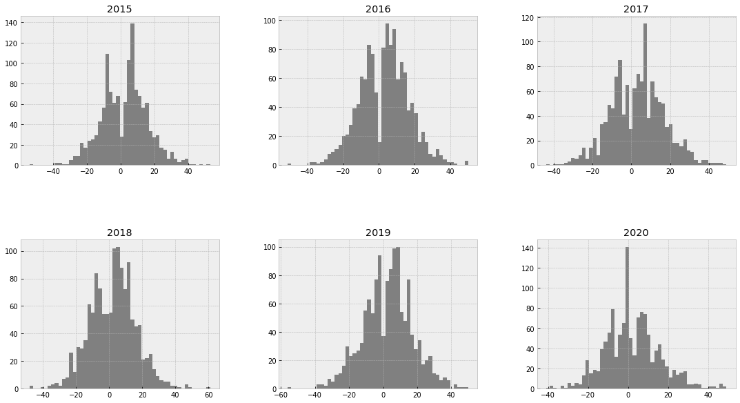
We can also visualize the overall distribution of the score differentials between the home and away teams across different seasons:
ax = (
    winloss_data
    .hist(
        by='year',
        column = 'score_diff',
        bins=50,
        figsize=(18, 10),
        layout=(2, 3),
        color='grey',
        rot=0
    )
)
The distribution of the score differentials between the home and away teams also displays some interesting patterns. The distributions for seasons 2015-2019 appear to follow a bi-modal distribution, with two spikes around zero (there is no such thing as a draw in basketball). In all cases, the “positive” spike is larger than the “negative” spike, which aligns with the previous observation that home teams were more likely to win their games during those seasons. This bi-model distribution is not as clearly defined for the 2020 season, where instead we see a significantly larger “negative” spike, which indicates that home teams were more likely to lose their games during that season.
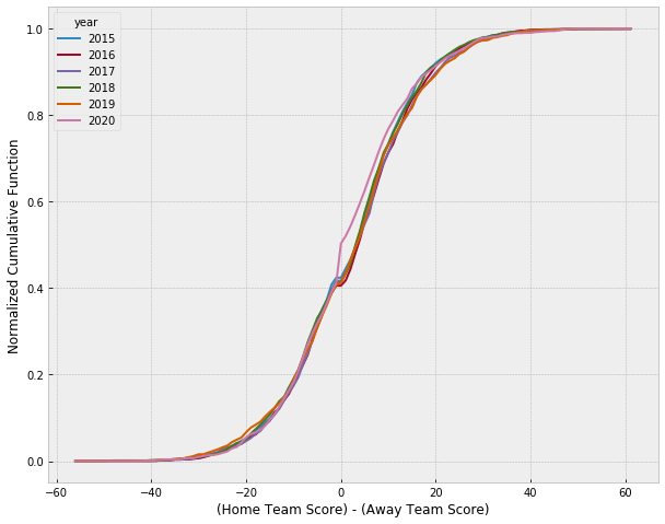
When plotting the normalized cumulative distribution function for the score differentials between the home and away teams, we obtain the following figure:
cum_score_diff = (
    winloss_data
    .groupby(['year', 'score_diff'])
    .size()
    .reset_index()
    .pivot(
        index='score_diff',
        columns='year',
        values=0
    )
    .fillna(0)
    .cumsum()
)

(cum_score_diff / cum_score_diff.max()).plot(figsize=(10, 8))
Again, the 2020 season stands apart from all other previous seasons included in our dataset, which shows a distinct uptick of games on the negative side of the zero mark that denotes games where the “away” team won. However, if we really want to show the potential impact of home-court advantage, we can focus on the before/after distribution of score differentials during the 2020 season. To begin, we define the months during games were played inside and outside of the bubble:
months_before_bubble = ['october', 'november', 'december', 'january', 'february']
months_after_bubble = ['july', 'august', 'september']
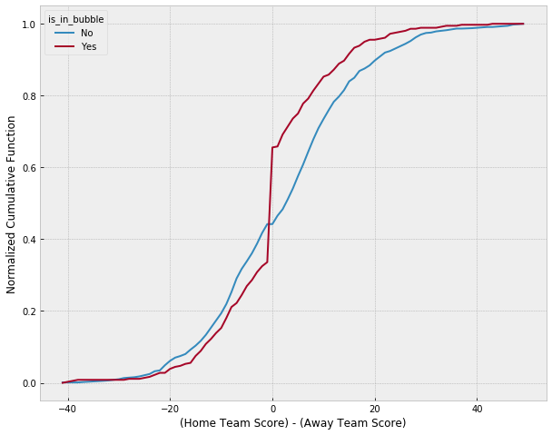
We can then compute and plot the normalized cumulative distribution function for the score differentials before and after the bubble:
cum_score_diff_2020 = (
    winloss_data
    .assign(
        is_in_bubble = ['No' if x in months_before else 'Yes' for x in winloss_data.month]
    )
    .query('year==2020')
    .groupby(['is_in_bubble', 'score_diff'])
    .size()
    .reset_index()
    .pivot(
        index='score_diff',
        columns='is_in_bubble',
        values=0
    )
    .fillna(0)
    .cumsum()
)

ax = (cum_score_diff_2020 / cum_score_diff_2020.max()).plot(figsize=(10, 8))
ax.set_xlabel('(Home Team Score) - (Away Team Score)')
ax.set_ylabel('Normalized Cumulative Function')
The figure clearly shows the impact that moving to a “bubble” environnment had on the score differentials between home and away teams. By entering a bubble in which all games were played on neutral arenas, the NBA negated the impact that fans could have on the outcome of games. As a result, we can reasonably conclude that the NBA bubble had a real impact on team performance, and that home-court advantage is a real phenomenom.